Python & Jupyter

Python Jupyter notebooks are an excellent way to experiment with data science and visualization. Using the higlass-jupyter extension, you can use HiGlass directly from within a Jupyter notebook.

Installation

To use higlass within a Jupyter notebook you need to install a few packages and enable the jupyter extension:

pip install jupyter higlass-python

jupyter nbextension install --py --sys-prefix --symlink higlass
jupyter nbextension enable --py --sys-prefix higlass

If you use JupyterLab you also have to run

jupyter labextension install @jupyter-widgets/jupyterlab-manager
jupyter labextension install higlass-jupyter

Uninstalling

jupyter nbextension uninstall --py --sys-prefix higlass

Examples

The examples below demonstrate how to use the HiGlass Python API to view data locally in a Jupyter notebook or a browser-based HiGlass instance.

For a fYou can find the demos from the talk at github.com/higlass/scipy19.

Jupyter HiGlass Component

To instantiate a HiGlass component within a Jupyter notebook, we first need to specify which data should be loaded. This can be accomplished with the help of the higlass.client module:

from higlass.client import View, Track
import higlass


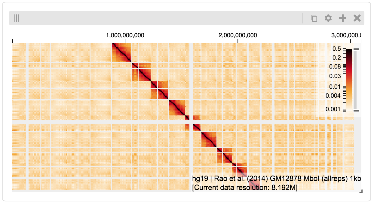
view1 = View([
    Track(track_type='top-axis', position='top'),
    Track(track_type='heatmap', position='center',
          tileset_uuid='CQMd6V_cRw6iCI_-Unl3PQ',
          server="http://higlass.io/api/v1/",
          height=250,
          options={ 'valueScaleMax': 0.5 }),
])

display, server, viewconf = higlass.display([view1])
display

The result is a fully interactive HiGlass view direcly embedded in the Jupyter notebook.

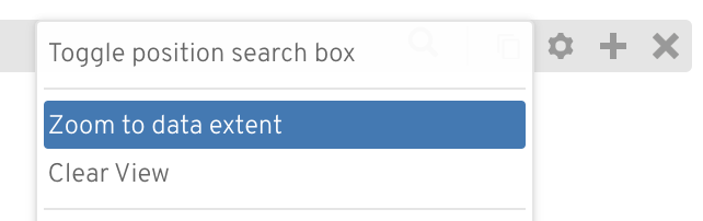
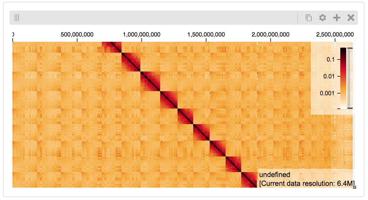
If the matrix doesn’t show up, you may have to click on “Zoom to data extent”:

Remote bigWig Files

bigWig files can be loaded either from the local disk or from remote http servers. The example below demonstrates how to load a remote bigWig file from the UCSC genome browser’s archives. Note that this is a network-heavy operation that may take a long time to complete with a slow internet connection.

from higlass.client import View, Track
import higlass.tilesets

ts1 = higlass.tilesets.bigwig(
    'http://hgdownload.cse.ucsc.edu/goldenpath/hg19/encodeDCC/'
    'wgEncodeSydhTfbs/wgEncodeSydhTfbsGm12878InputStdSig.bigWig')

tr1 = Track('horizontal-bar', tileset=ts1)
view1 = View([tr1])
display, server, viewconf = higlass.display([view1])

display

Serving local data

To view local data, we need to define the tilesets and set up a temporary server.

Cooler Files

Creating the server:

from higlass.client import View, Track
from higlass.tilesets import cooler
import higlass

ts1 = cooler('../data/Dixon2012-J1-NcoI-R1-filtered.100kb.multires.cool')
tr1 = Track('heatmap', tileset=ts1)
view1 = View([tr1])
display, server, viewconf = higlass.display([view1])

display

BigWig Files

In this example, we’ll set up a server containing both a chromosome labels track and a bigwig track. Furthermore, the bigwig track will be ordered according to the chromosome info in the specified file.

from higlass.client import View, Track
from higlass.tilesets import bigwig, chromsizes
import higlass.tilesets

chromsizes_fp = '../data/chromSizes_hg19_reordered.tsv'
bigwig_fp = '../data/wgEncodeCaltechRnaSeqHuvecR1x75dTh1014IlnaPlusSignalRep2.bigWig'

with open(chromsizes_fp) as f:
    chromsizes = []
    for line in f.readlines():
        chrom, size = line.split('\t')
        chromsizes.append((chrom, int(size)))

cs = chromsizes(chromsizes)
ts = bigwig(bigwig_fp, chromsizes=chromsizes)

tr0 = Track('top-axis')
tr1 = Track('horizontal-bar', tileset=ts)
tr2 = Track('horizontal-chromosome-labels', position='top', tileset=cs)

view1 = View([tr0, tr1, tr2])
display, server, viewconf = higlass.display([view1])

display

The client view will be composed such that three tracks are visible. Two of them are served from the local server.

Serving custom data

To display data, we need to define a tileset. Tilesets define two functions: tileset_info:

> from higlass.tilesets import bigwig
> ts1 = bigwig('http://hgdownload.cse.ucsc.edu/goldenpath/hg19/encodeDCC/wgEncodeSydhTfbs/wgEncodeSydhTfbsGm12878InputStdSig.bigWig')
> ts1.tileset_info()
{
 'min_pos': [0],
 'max_pos': [4294967296],
 'max_width': 4294967296,
 'tile_size': 1024,
 'max_zoom': 22,
 'chromsizes': [['chr1', 249250621],
                ['chr2', 243199373],
                ...],
 'aggregation_modes': {'mean': {'name': 'Mean', 'value': 'mean'},
                       'min': {'name': 'Min', 'value': 'min'},
                       'max': {'name': 'Max', 'value': 'max'},
                       'std': {'name': 'Standard Deviation', 'value': 'std'}},
 'range_modes': {'minMax': {'name': 'Min-Max', 'value': 'minMax'},
                 'whisker': {'name': 'Whisker', 'value': 'whisker'}}
 }

and tiles:

> ts1.tiles(['x.0.0'])
[('x.0.0',
  {'min_value': 0.0,
   'max_value': 9.119079544037932,
   'dense': 'Rh25PwcCcz...',   # base64 string encoding the array of data
   'size': 1,
   'dtype': 'float32'})]

The tiles function will always take an array of tile ids of the form id.z.x[.y][.transform] where z is the zoom level, x is the tile’s x position, y is the tile’s y position (for 2D tilesets) and transform is some transform to be applied to the data (e.g. normalization types like ice).

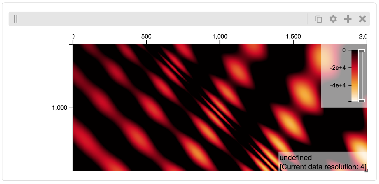
Numpy Matrix

By way of example, let’s explore a numpy matrix by implementing the tileset_info and tiles functions described above. To start let’s make the matrix using the Eggholder function.

import numpy as np

dim = 2000
I, J = np.indices((dim, dim))
data = (
    -(J + 47) * np.sin(np.sqrt(np.abs(I / 2 + (J + 47))))
    - I * np.sin(np.sqrt(np.abs(I - (J + 47))))
)

Then we can define the data and tell the server how to render it.

from  clodius.tiles import npmatrix
from higlass.tilesets import Tileset

ts = Tileset(
    tileset_info=lambda: npmatrix.tileset_info(data),
    tiles=lambda tids: npmatrix.tiles_wrapper(data, tids)
)

display, server, viewconf = higlass.display([
    View([
        Track(track_type='top-axis', position='top'),
        Track(track_type='left-axis', position='left'),
        Track(track_type='heatmap',
              position='center',
              tileset=ts,
              height=250,
              options={ 'valueScaleMax': 0.5 }),

    ])
])
display

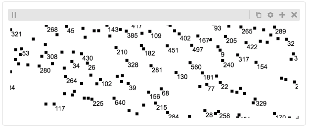
Displaying Many Points

To display, for example, a list of 1 million points in a HiGlass window inside of a Jupyter notebook. First we need to import the custom track type for displaying labelled points:

%%javascript

require(["https://unpkg.com/higlass-labelled-points-track@0.1.11/dist/higlass-labelled-points-track"],
    function(hglib) {

});

Then we have to set up a data server to output the data in “tiles”.

import numpy as np
import pandas as pd
from higlass.client import View, Track
from higlass.tilesets import dfpoints

length = int(1e6)
df = pd.DataFrame({
    'x': np.random.random((length,)),
    'y': np.random.random((length,)),
    'v': range(1, length+1),
})

ts = dfpoints(df, x_col='x', y_col='y')

display, server, viewconf = higlass.display([
    View([
        Track('left-axis'),
        Track('top-axis'),
        Track('labelled-points-track',
               tileset=ts,
               position='center',
               height=600,
               options={
                    'xField': 'x',
                    'yField': 'y',
                    'labelField': 'v'
        }),
    ])
])

display

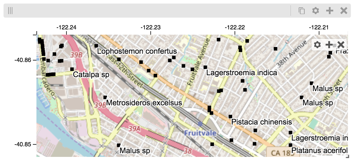
This same technique can be used to display points in a GeoJSON file. First we have to extract the values from the GeoJSON file and create a dataframe:

import math

def lat2y(a):
  return 180.0/math.pi*math.log(math.tan(math.pi/4.0+a*(math.pi/180.0)/2.0))

x = [t['geometry']['coordinates'][0] for t in trees['features']]
y = [-lat2y(t['geometry']['coordinates'][1]) for t in trees['features']]
names = [t['properties']['SPECIES'] for t in trees['features']]

df = pd.DataFrame({ 'x': x, 'y': y, 'names': names })
df = df.sample(frac=1).reset_index(drop=True)

And then create the tileset and track, as before.

from higlass.client import View, Track
from higlass.tilesets import dfpoints

ts = dfpoints(df, x_col='x', y_col='y')

display, server, viewconf = higlass.display([
    View([
        Track('left-axis'),
        Track('top-axis'),
        Track('osm-tiles', position='center'),
        Track('labelled-points-track',
               tileset=ts,
               position='center',
               height=600,
               options={
                    'xField': 'x',
                    'yField': 'y',
                    'labelField': 'names'
        }),
    ])
])

display

Other constructs

The examples containing dense data above use the bundled_tiles_wrapper_2d function to translate lists of tile_ids to tile data. This consolidates tiles that are within rectangular blocks and fulfills them simultaneously. The return type is a list of (tile_id, formatted_tile_data) tuples.

In cases where we don’t have such a function handy, there’s the simpler tiles_wrapper_2d which expects the target to fullfill just single tile requests:

from clodius.tiles.format import format_dense_tile
from clodius.tiles.utils import tiles_wrapper_2d
from higlass.tilesets import Tileset

ts = Tileset(
    tileset_info=tileset_info,
    tiles=lambda tile_ids: tiles_wrapper_2d(tile_ids,
                    lambda z,x,y: format_dense_tile(tile_data(z, x, y)))
)

In this case, we expect tile_data to simply return a matrix of values.